

Powered by Open Source CGL MOOC Builder Technology built on Google Course Builder

Instructor
Professor Geoffrey Fox received a PhD in Theoretical Physics from Cambridge University and is now Professor of Informatics and Computing as well as Physics at Indiana University, where he is director of the Digital Science Center and Associate Dean for Research and Graduate Studies at the School of Informatics and Computing. He previously held positions at Caltech, Syracuse University and Florida State University.
He has published around 1,000 papers in Physics and Computer Science, supervised the PhD candidacies of 65 students, and received an h-index of 67 along with over 23000 citations. Professor Fox currently works in applying Computer Science to Bioinformatics, Sensor Clouds, Earthquake and Ice-sheet Science, and Particle Physics. He is principal investigator of FutureGrid – a facility to enable development of new approaches to computing. He is involved in several projects, including the eHumanity portal, to enhance the capability of Minority Serving Institutions. A Fellow of APS and ACM, he has experience in online education and its use in MOOCs for areas like Data and Computational Science.
This section has a technical overview of course followed by a broad motivation for course.
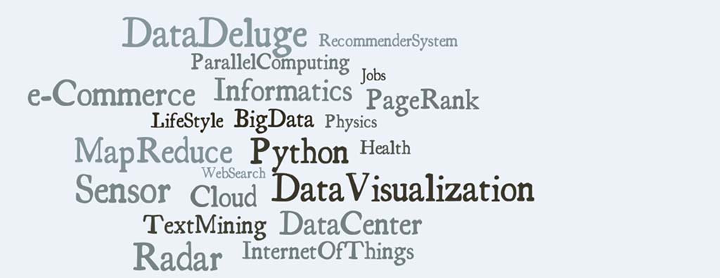
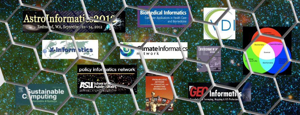
The course overview covers it's content and structure. It presents the X-Informatics fields (defined values of X) and the Rallying cry of course: Use Clouds running Data Analytics Collaboratively processing Big Data to solve problems in X-Informatics ( or e-X). The courses is set up as a MOOC divided into units that vary in length but are typically around an hour and those are further subdivided into 5-15 minute lessons. The course covers a mix of applications (the X in X-Informatics) and technologies needed to support the field electronically i.e. to process the application data. The overview ends with a discussion of course content at highest level. The course starts with a longish Motivation unit summarizing clouds and data science, then units describing applications (X = Physics, e-Commerce, Web Search and Text mining, Health, Sensors and Remote Sensing). These are interspersed with discussions of infrastructure (clouds) and data analytics (algorithms like clustering and collaborative filtering used in applications). The course uses either Python or Java and there are Side MOOCs discussing Python and Java tracks.
The course motivation starts with striking examples of the data deluge with examples from research, business and the consumer. The growing number of jobs in data science is highlighted. He describes industry trend in both clouds and big data. Then the cloud computing model developed at amazing speed by industry is introduced. The 4 paradigms of scientific research are described with growing importance of data oriented version.He covers 3 major X-informatics areas: Physics, e-Commerce and Web Search followed by a broad discussion of cloud applications. Parallel computing in general and particular features of MapReduce are described. He comments on a data science education and the benefits of using MOOC's.
Geoffrey gives a short introduction to the course covering its content and structure. He presents the X-Informatics fields (defined values of X) and the Rallying cry of course: Use Clouds running Data Analytics Collaboratively processing Big Data to solve problems in X-Informatics (or e-X). The courses is set up as a MOOC divided into units that vary in length but are typically around an hour and those are further subdivided into 5-15 minute lessons.
The course covers a mix of applications (the X in X-Informatics) and technologies needed to support the field electronically i.e. to process the application data. The introduction ends with a discussion of course content at highest level.
The course starts with a longish Motivation unit summarizing clouds and data science, then units describing applications (X = Physics, e-Commerce, Web Search and Text mining, Health, Sensors and Remote Sensing). These are interspersed with discussions of infrastructure (clouds) and data analytics (algorithms like clustering and collaborative filtering used in applications)
The course uses either Python or Java and there are Side MOOCs discussing Python and Java tracks.
Geoffrey gives a short introduction to the course covering it's content and structure. He presents the X-Informatics fields (defined values of X) and the Rallying cry of course: Use Clouds running Data Analytics Collaboratively processing Big Data to solve problems in X-Informatics ( or e-X). The courses is set up as a MOOC divided into units that vary in length but are typically around an hour and those are further subdivided into 5-15 minute lessons. Geoffrey follows discussion of mechanics of course with a list of all the units offered
This course gives an overview of big data from a use case (application) point of view noting that big data in field X drives the concept of X-Informatics. It covers applications, algorithms and infrastructure/technology (cloud computing). There are 3 versions of Spring 2014 course: I400 Informatics at IU for Undergraduates, I590 Informatics at IU for Graduate students, I590 component of non residential data science certificate. They differ in homework and recommended/required lectures. A single web resource handles lectures for all 3 classes
Geoffrey discusses some of the available units:
Motivation: Big Data and the Cloud; Centerpieces of the Future Economy
Introduction: What is Big Data, Data Analytics and X-Informatics
Python for Big Data Applications and Analytics: NumPy, SciPy, MatPlotlib
Using FutureGrid for Big Data Applications and Analytics Course
X-Informatics Physics Use Case, Discovery of Higgs Particle; Counting Events and Basic Statistics Parts I-IV
Geoffrey discusses some more of the available units:X-Informatics Use Cases: Big Data Use Cases Survey
Using Plotviz Software for Displaying Point Distributions in 3D
X-Informatics Use Case: e-Commerce and Lifestyle with recommender systems
Technology Recommender Systems - K-Nearest Neighbors, Clustering and heuristic methods
Parallel Computing Overview and familiar examples
Cloud Technology for Big Data Applications & Analytics
Geoffrey discusses the remainder of the available units:
X-Informatics Use Case: Web Search and Text Mining and their technologies
Technology for X-Informatics: PageRank
Technology for X-Informatics: Kmeans
Technology for X-Informatics: MapReduce
Technology for X-Informatics: Kmeans and MapReduce Parallelism
X-Informatics Use Case: Sports
X-Informatics Use Case: Health
X-Informatics Use Case: Sensors
X-Informatics Use Case: Radar for Remote Sensing.
Geoffrey motivates the study of X-informatics by describing data science and clouds. He starts with striking examples of the data deluge with examples from research, business and the consumer. The growing number of jobs in data science is highlighted. He describes industry trend in both clouds and big data.
He introduces the cloud computing model developed at amazing speed by industry. The 4 paradigms of scientific research are described with growing importance of data oriented version. He covers 3 major X-informatics areas: Physics, e-Commerce and Web Search followed by a broad discussion of cloud applications. Parallel computing in general and particular features of MapReduce are described. He comments on a data science education and the benefits of using MOOC's.
This presents the overview of talk, some trends in computing and data and jobs. Gartner's emerging technology hype cycle shows many areas of Clouds and Big Data. Geoffrey highlights 6 issues of importance: economic imperative, computing model, research model, Opportunities in advancing computing, Opportunities in X-Informatics, Data Science Education
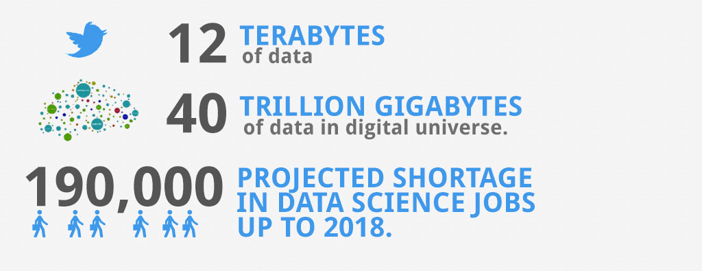
Geoffrey gives some amazing statistics for total storage; uploaded video and uploaded photos; the social media interactions every minute; aspects of the business big data tidal wave; monitors of aircraft engines; the science research data sizes from particle physics to astronomy and earth science; genes sequenced; and finally the long tail of science. The next slide emphasizes applications using algorithms on clouds. This leads to the rallying cry ''Use Clouds running Data Analytics Collaboratively processing Big Data to solve problems in X-Informatics educated in data science'' with a catalog of the many values of X ''Astronomy, Biology, Biomedicine, Business, Chemistry, Climate, Crisis, Earth Science, Energy, Environment, Finance, Health, Intelligence, Lifestyle, Marketing, Medicine, Pathology, Policy, Radar, Security, Sensor, Social, Sustainability, Wealth and Wellness''
Jobs abound in clouds and data science. There are documented shortages in data science, computer science and the major tech companies advertise for new talent.
Trends include the growing importance of mobile devices and comparative decrease in desktop access, the export of internet content, the change in dominant client operating systems, use of social media, thriving chinese internet companies
Not everything goes up. The rise of the Internet has led to declines in some traditional areas including Shopping malls and Postal Services.
Clouds and Big Data are transformational on a 2-5 year time scale. Already Amazon AWS is a lucrative business with almost a $4B revenue. Geoffrey describes the nature of cloud centers with economies of scale and gives examples of importance of virtualization in server consolidation. Then key characteristics of clouds are reviewed with expected high growth in Infrastructure, Platform and Software as a Service.
Geoffrey introduces the 4 paradigms of scientific research with the focus on the new fourth data driven methodology.
Geoffrey introduces the DIKW data to information to knowledge to wisdom paradigm. Data flows through cloud services transforming itself and emerging as new information to input into other transformations.
Geoffrey looks at important particle physics example where the Large hadron Collider has observed the Higgs Boson. He shows this discovery as a bump in a histogram; something that so amazed him 50 years ago that he got a PhD in this field. He left field partly due to the incredible size of author lists on papers
Many important applications involve matching users, web pages, jobs, movies, books, events etc. These are all optimization problems with recommender systems one important way of performing this optimization. Geoffrey goes through the example of Netflix -- everything is a recommendation and muses about the power of viewing all sorts of things as items in a bag or more abstractly some space with funny properties
Many important applications involve matching users, web pages, jobs, movies, books, events etc. These are all optimization problems with recommender systems one important way of performing this optimization. Geoffrey goes through the example of Netflix -- everything is a recommendation and muses about the power of viewing all sorts of things as items in a bag or more abstractly some space with funny properties
This course also looks at Web Search and here Geoffrey gives an overview of the data analytics for web search, Pagerank as a method of ranking web pages returned and uses material from Yahoo on the subtle algorithms for dynamic personalized choice of material for web pages.
Geoffrey describes scientific applications and how they map onto clouds, supercomputers, grids and high throughput systems. He likes the cloud use of the Internet of Things and gives examples.
Geoffrey defines MapReduce and gives a homely example from fruit blending.
Geoffrey discusses one reason you are taking this course -- Data Science as an educational initiative and aspects of its Indiana University implementation. Then general; features of online education are discussed with clear growth spearheaded by MOOC's where Geoffrey uses this course and others as an example. He stresses the choice between one class to 100,000 students or 2,000 classes to 50 students and an online library of MOOC lessons. In olden days he suggested ''hermit's cage virtual university'' -- gurus in isolated caves putting together exciting curricula outside the traditional university model. Grading and mentoring models and important online tools are discussed. Clouds have MOOC's describing them and MOOC's are stored in clouds; a pleasing symmetry.
The conclusions highlight clouds, data-intensive methodology, employment, data science, MOOC's and never forget the Big Data ecosystem in one sentence ''Use Clouds running Data Analytics Collaboratively processing Big Data to solve problems in X-Informatics educated in data science''
The course introduction starts with X-Informatics and its rallying cry. The growing number of jobs in data science is highlighted. The first unit offers a look at the phenomenon described as the Data Deluge starting with its broad features. Data science and the famous DIKW (Data to Information to Knowledge to Wisdom) pipeline are covered. Then more detail is given on the flood of data from Internet and Industry applications with eBay and General Electric discussed in most detail.
In the next unit, Geoffrey continues the discussion of the data deluge with a focus on scientific research. He takes a first peek at data from the Large Hadron Collider considered later as physics Informatics and gives some biology examples. He discusses the implication of data for the scientific method which is changing with the data-intensive methodology joining observation, theory and simulation as basic methods. Two broad classes of data are the long tail of sciences: many users with individually modest data adding up to a lot; and a myriad of Internet connected devices -- the Internet of Things.
Geoffrey gives an initial technical overview of cloud computing as pioneered by companies like Amazon, Google and Microsoft with new centers holding up to a million servers. The benefits of Clouds in terms of power consumption and the environment are also touched upon, followed by a list of the most critical features of Cloud computing with a comparison to supercomputing. Features of the data deluge are discussed with a salutary example where more data did better than more thought. Then comes Data science and one part of it -- data analytics -- the large algorithms that crunch the big data to give big wisdom. There are many ways to describe data science and several are discussed to give a good composite picture of this emerging field.
Geoffrey starts with X-Informatics and its rallying cry. The growing number of jobs in data science is highlighted. This unit offers a look at the phenomenon described as the Data Deluge starting with its broad features. Then he discusses data science and the famous DIKW (Data to Information to Knowledge to Wisdom) pipeline. Then more detail is given on the flood of data from Internet and Industry applications with eBay and General Electric discussed in most detail.
This discusses trends that are driven by and accompany Big data. We give some key terms including data, information, knowledge, wisdom, data analytics and data science. WE introduce the motto of the course: Use Clouds running Data Analytics Collaboratively processing Big Data to solve problems in X-Informatics. We list many values of X you can defined in various activities across the world.
Big data is especially important as there are some many related jobs. We illustrate this for both cloud computing and data science from reports by Microsoft and the McKinsey institute respectively. We show a plot from LinkedIn showing rapid increase in the number of data science and analytics jobs as a function of time.
We look at some broad features of the data deluge starting with the size of data in various areas especially in science research. We give examples from real world of the importance of big data and illustrate how it is integrated into an enterprise IT architecture. We give some views as to what characterizes Big data and why data science is a science that is needed to interpret all the data.
We stress the DIKW pipeline: Data becomes information that becomes knowledge and then wisdom, policy and decisions. This pipeline is illustrated with Google maps and we show how complex the ecosystem of data, transformations (filters) and its derived forms is.
We give examples of Big data from the Internet with Tweets, uploaded photos and an illustration of the vitality and size of many commodity applications.
We give examples including the Big data that enables wind farms, city transportation, telephone operations, machines with health monitors, the banking, manufacturing and retail industries both online and offline in shopping malls. We give examples from ebay showing how analytics allowing them to refine and improve the customer experiences.
We give examples including the Big data that enables wind farms, city transportation, telephone operations, machines with health monitors, the banking, manufacturing and retail industries both online and offline in shopping malls. We give examples from ebay showing how analytics allowing them to refine and improve the customer experiences.
We give examples including the Big data that enables wind farms, city transportation, telephone operations, machines with health monitors, the banking, manufacturing and retail industries both online and offline in shopping malls. We give examples from ebay showing how analytics allowing them to refine and improve the customer experiences.
Geoffrey continues the discussion of the data deluge with a focus on scientific research. He takes a first peek at data from the Large Hadron Collider considered later as physics Informatics and gives some biology examples. He discusses the implication of data for the scientific method which is changing with the data-intensive methodology joining observation, theory and simulation as basic methods.
We discuss the long tail of sciences; many users with individually modest data adding up to a lot. The last lesson emphasizes how everyday devices -- the Internet of Things -- are being used to create a wealth of data.
We look into more big data examples with a focus on science and research. We give astronomy, genomics, radiology, particle physics and discovery of Higgs particle (Covered in more detail in later lessons), European Bioinformatics Institute and contrast to Facebook and Walmart
We look into more big data examples with a focus on science and research. We give astronomy, genomics, radiology, particle physics and discovery of Higgs particle (Covered in more detail in later lessons), European Bioinformatics Institute and contrast to Facebook and Walmart
We discuss the emergences of a new fourth methodology for scientific research based on data driven inquiry. We contrast this with third -- computation or simulation based discovery - methodology which emerged itself some 25 years ago.
There is big science such as particle physics where a single experiment has 3000 people collaborate!.Then there are individual investigators who don't generate a lot of data each but together they add up to Big data.
A final category of Big data comes from the Internet of Things where lots of small devices -- smart phones, web cams, video games collect and disseminate data and are controlled and coordinated in the cloud
Geoffrey gives an initial technical overview of cloud computing as pioneered by companies like Amazon, Google and Microsoft with new centers holding up to a million servers. The benefits of Clouds in terms of power consumption and the environment are also touched upon, followed by a list of the most critical features of Cloud computing with a comparison to supercomputing.
He discusses features of the data deluge with a salutary example where more data did better than more thought. He introduces data science and one part of it -- data analytics -- the large algorithms that crunch the big data to give big wisdom. There are many ways to describe data science and several are discussed to give a good composite picture of this emerging field.
We describe cloud data centers with their staggering size with up to a million servers in a single data center and centers built modularly from shipping containers full of racks. The benefits of Clouds in terms of power consumption and the environment are also touched upon, followed by a list of the most critical features of Cloud computing and a comparison to supercomputing.
Data, Information, intelligence algorithms, infrastructure, data structure, semantics and knowledge are related. The semantic web and Big data are compared. We give an example where ''More data usually beats better algorithms''. We discuss examples of intelligent big data and list 8 different types of data deluge
Data, Information, intelligence algorithms, infrastructure, data structure, semantics and knowledge are related. The semantic web and Big data are compared. We give an example where ''More data usually beats better algorithms''. We discuss examples of intelligent big data and list 8 different types of data deluge
We describe and critique one view of the work of a data scientists. Then we discuss and contrast 7 views of the process needed to speed data through the DIKW pipeline.
We stress the importance of data analytics giving examples from several fields. We note that better analytics is as important as better computing and storage capability.
We stress the importance of data analytics giving examples from several fields. We note that better analytics is as important as better computing and storage capability.

This section is meant to give an overview of the python tools needed for doing for this course. These are really powerful tools which every data scientist who wishes to use python must know. This section covers. Canopy - Its is an IDE for python developed by EnThoughts. The aim of this IDE is to bring the various python libraries under one single framework or ''Canopy'' - that is why the name. NumPy - It is popular library on top of which many other libraries (like pandas, scipy) are built. It provides a way a vectorizing data. This helps to organize in a more intuitive fashion and also helps us use the various matrix operations which are popularly used by the machine learning community. Matplotlib: This a data visualization package. It allows you to create graphs charts and other such diagrams. It supports Images in JPEG, GIF, TIFF format. SciPy: SciPy is a library built above numpy and has a number of off the shelf algorithms / operations implemented. These include algorithms from calculus(like integration), statistics, linear algebra, image-processing, signal processing, machine learning, etc.
This section is meant to give an overview of the python tools needed for doing for this course. These are really powerful tools which every data scientist who wishes to use python must know.
This section is meant to give an overview of the python tools needed for doing for this course. These are really powerful tools which every data scientist who wishes to use python must know. This section covers Canopy, NumPy, MatPlotLib, and Scipy.
Canopy - Its is an IDE for python developed by EnThoughts. The aim of this IDE is to bring the various python libraries under one single framework or ''Canopy'' - that is why the name.
NumPy - It is popular library on top of which many other libraries (like pandas, scipy) are built. It provides a way a vectorizing data. This helps to organize in a more intuitive fashion and also helps us use the various matrix operations which are popularly used by the machine learning community.
NumPy - It is popular library on top of which many other libraries (like pandas, scipy) are built. It provides a way a vectorizing data. This helps to organize in a more intuitive fashion and also helps us use the various matrix operations which are popularly used by the machine learning community.
NumPy - It is popular library on top of which many other libraries (like pandas, scipy) are built. It provides a way a vectorizing data. This helps to organize in a more intuitive fashion and also helps us use the various matrix operations which are popularly used by the machine learning community.
Matplotlib: This a data visualization package. It allows you to create graphs charts and other such diagrams. It supports Images in JPEG, GIF, TIFF format.
Matplotlib: This a data visualization package. It allows you to create graphs charts and other such diagrams. It supports Images in JPEG, GIF, TIFF format.
SciPy: SciPy is a library built above numpy and has a number of off the shelf algorithms / operations implemented. These include algorithms from calculus(like integration), statistics, linear algebra, image-processing, signal processing, machine learning, etc.
SciPy: SciPy is a library built above numpy and has a number of off the shelf algorithms / operations implemented. These include algorithms from calculus(like integration), statistics, linear algebra, image-processing, signal processing, machine learning, etc.
This section is meant to give an overview of the Future Grid and how to use for the Big Data Course. In addition to this creating FutureGrid Account, Uploading OpenId and SSH Key and how to instantiate and log into Virtual Machine and accessing Ipython are covered. In the end we discuss about running Python and Java on Virtual Machine.
In this video Geoffrey introduces Future Grid in terms of its services and features
This lesson explains how to create a portal account, which is the first step in gaining access to FutureGrid
This lesson explains how to upload and use OpenID to easily log into the FutureGrid portal.
This lesson explains how to upload and use a SSH key to log to the FutureGrid resources
This lesson explains how to join a FutureSystems project. For this class please joing project number 455.
This lesson explains how to log into FG and our customized shell and menu options that will simplify management of the VMs for this upcoming lessons.
This lesson explains about Running Java and Python on FG
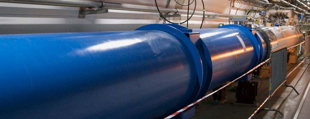
This section starts by describing the LHC accelerator at CERN and evidence found by the experiments suggesting existence of a Higgs Boson. The huge number of authors on a paper, remarks on histograms and Feynman diagrams is followed by an accelerator picture gallery. The next unit is devoted to Python experiments looking at histograms of Higgs Boson production with various forms of shape of signal and various background and with various event totals. Then random variables and some simple principles of statistics are introduced with explanation as to why they are relevant to Physics counting experiments. The unit introduces Gaussian (normal) distributions and explains why they seen so often in natural phenomena. Several Python illustrations are given. Random Numbers with their Generators and Seeds lead to a discussion of Binomial and Poisson Distribution. Monte-Carlo and accept-reject methods. The Central Limit Theorem concludes discussion.
This unit is devoted to Python and Java experiments with Geoffrey looking at histograms of Higgs Boson production with various forms of shape of signal and various background and with various event totals. The lectures use Python but use of Java is described.
We return to particle case with slides used in introduction and stress that particles often manifested as bumps in histograms and those bumps need to be large enough to stand out from background in a statistically significant fashion.
We give a few details on one LHC experiment ATLAS. Experimental physics papers have a staggering number of authors and quite big budgets. Feynman diagrams describe processes in a fundamental fashion.
We give a few details on one LHC experiment ATLAS. Experimental physics papers have a staggering number of authors and quite big budgets. Feynman diagrams describe processes in a fundamental fashion.
This lesson gives a small picture gallery of accelerators. Accelerators, detection chambers and magnets in tunnels and a large underground laboratory used fpr experiments where you need to be shielded from background like cosmic rays
This unit is devoted to Python experiments with Geoffrey looking at histograms of Higgs Boson production with various forms of shape of signal and various background and with various event totals
We discuss how this unit uses Java and Python on both a backend server (FutureGrid) or a local client. WE point out useful book on Python for data analysis. This builds on technology training in Section 3
We define ''event counting'' data collection environments. We discuss the python and Java code to generate events according to a particular scenario (the important idea of Monte Carlo data). Here a sloping background plus either a Higgs particle generated similarly to LHC observation or one observed with better resolution (smaller measurement error).
This uses Monte Carlo data both to generate data like the experimental observations and explore effect of changing amount of data and changing measurement resolution for Higgs.
This lesson continues the examination of Monte Carlo data looking at effect of change in number of Higgs particles produced and in change in shape of background
Geoffrey introduces random variables and some simple principles of statistics and explains why they are relevant to Physics counting experiments. The unit introduces Gaussian (normal) distributions and explains why they seen so often in natural phenomena. Several Python illustrations are given. Java is currently not available in this unit.
We go through the many different areas of statistics covered in the Physics unit. We define the statistics concept of a random variable.
We describe the DIKW pipeline for the analysis of this type of physics experiment and go through details of analysis pipeline for the LHC ATLAS experiment. We give examples of event displays showing the final state particles seen in a few events. We illustrate how physicists decide whats going on with a plot of expected Higgs production experimental cross sections (probabilities) for signal and background.
We describe the DIKW pipeline for the analysis of this type of physics experiment and go through details of analysis pipeline for the LHC ATLAS experiment. We give examples of event displays showing the final state particles seen in a few events. We illustrate how physicists decide whats going on with a plot of expected Higgs production experimental cross sections (probabilities) for signal and background.
We introduce Poisson and Binomial distributions and define independent identically distributed (IID) random variables. We give the law of large numbers defining the errors in counting and leading to Gaussian distributions for many things. We demonstrate this in Python experiments.
We introduce the Gaussian distribution and give Python examples of the fluctuations in counting Gaussian distributions.
We discuss the significance of a standard deviation and role of biases and insufficient statistics with a Python example in getting incorrect answers.
Geoffrey discusses Random Numbers with their Generators and Seeds. It introduces Binomial and Poisson Distribution. Monte-Carlo and accept-reject methods are discussed. The Central Limit Theorem and Bayes law concludes discussion. Python and Java (for student - not reviewed in class) examples and Physics applications are given.
We define random numbers and describe how to generate them on the computer giving Python examples. We define the seed used to define to specify how to start generation.
We define random numbers and describe how to generate them on the computer giving Python examples. We define the seed used to define to specify how to start generation.
We define binomial distribution and give LHC data as an eaxmple of where this distribution valid.
We introduce an advanced method -- accept/reject -- for generating random variables with arbitrary distrubitions.
We define Monte Carlo method which usually uses accept/reject method in typical case for distribution.
We extend the Binomial to the Poisson distribution and give a set of amusing examples from Wikipedia.
We introduce Central Limit Theorem and give examples from Wikipedia.
This lesson describes difference between Bayes and frequency views of probability. Bayes's law of conditional probability is derived and applied to Higgs example to enable information about Higgs from multiple channels and multiple experiments to be accumulated.
This section covers 51 values of X and an overall study of Big data that emerged from a NIST (National Institute for Standards and Technology) study of Big data. The section covers the NIST Big Data Public Working Group (NBD-PWG) Process and summarizes the work of five subgroups: Definitions and Taxonomies Subgroup, Reference Architecture Subgroup, Security and Privacy Subgroup, Technology Roadmap Subgroup and the Requirements andUse Case Subgroup. 51 use cases collected in this process are briefly discussed with a classification of the source of parallelism and the high and low level computational structure. We describe the key features of this classification.
This unit covers the NIST Big Data Public Working Group (NBD-PWG) Process and summarizes the work of five subgroups: Definitions and Taxonomies Subgroup, Reference Architecture Subgroup, Security and Privacy Subgroup, Technology Roadmap Subgroup and the Requirements and Use Case Subgroup. The work of latter is continued in next two units.
The focus of the (NBD-PWG) is to form a community of interest from industry, academia, and government, with the goal of developing a consensus definitions, taxonomies, secure reference architectures, and technology roadmap. The aim is to create vendor-neutral, technology and infrastructure agnostic deliverables to enable big data stakeholders to pick-and-choose best analytics tools for their processing and visualization requirements on the most suitable computing platforms and clusters while allowing value-added from big data service providers and flow of data between the stakeholders in a cohesive and secure manner.
The focus is to gain a better understanding of the principles of Big Data. It is important to develop a consensus-based common language and vocabulary terms used in Big Data across stakeholders from industry, academia, and government. In addition, it is also critical to identify essential actors with roles and responsibility, and subdivide them into components and sub-components on how they interact/ relate with each other according to their similarities and differences.
For Definitions: Compile terms used from all stakeholders regarding the meaning of Big Data from various standard bodies, domain applications, and diversified operational environments. For Taxonomies: Identify key actors with their roles and responsibilities from all stakeholders, categorize them into components and subcomponents based on their similarities and differences. In particular data Science and Big Data terms are discussed
The focus is to form a community of interest from industry, academia, and government, with the goal of developing a consensus-based approach to orchestrate vendor-neutral, technology and infrastructure agnostic for analytics tools and computing environments. The goal is to enable Big Data stakeholders to pick-and-choose technology-agnostic analytics tools for processing and visualization in any computing platform and cluster while allowing value-added from Big Data service providers and the flow of the data between the stakeholders in a cohesive and secure manner. Results include a reference architecture with well defined components and linkage as well as several exemplars
The focus is to form a community of interest from industry, academia, and government, with the goal of developing a consensus secure reference architecture to handle security and privacy issues across all stakeholders. This includes gaining an understanding of what standards are available or under development, as well as identifies which key organizations are working on these standards. The Top Ten Big Data Security and Privacy Challenges from the CSA (Cloud Security Alliance) BDWG are studied. Specialized use cases include Retail/Marketing, Modern Day Consumerism, Nielsen Homescan, Web Traffic Analysis, Healthcare, Health Information Exchange, Genetic Privacy, Pharma Clinical Trial Data Sharing, Cyber-security, Government, Military and Education.
The focus is to form a community of interest from industry, academia, and government, with the goal of developing a consensus vision with recommendations on how Big Data should move forward by performing a good gap analysis through the materials gathered from all other NBD subgroups. This includes setting standardization and adoption priorities through an understanding of what standards are available or under development as part of the recommendations. Tasks are gather input from NBD subgroups and study the taxonomies for the actors' roles and responsibility, use cases and requirements, and secure reference architecture; gain understanding of what standards are available or under development for Big Data; perform a thorough gap analysis and document the findings; identify what possible barriers may delay or prevent adoption of Big Data; and document vision and recommendations.
The focus is to form a community of interest from industry, academia, and government, with the goal of developing a consensus list of Big Data requirements across all stakeholders. This includes gathering and understanding various use cases from diversified application domains.Tasks are gather use case input from all stakeholders; derive Big Data requirements from each use case; analyze/prioritize a list of challenging general requirements that may delay or prevent adoption of Big Data deployment; develop a set of general patterns capturing the ''essence'' of use cases (not done yet) and work with Reference Architecture to validate requirements and reference architecture by explicitly implementing some patterns based on use cases. The progress of gathering use cases (discussed in next two units) and requirements systemization are discussed.
The focus is to form a community of interest from industry, academia, and government, with the goal of developing a consensus list of Big Data requirements across all stakeholders. This includes gathering and understanding various use cases from diversified application domains.Tasks are gather use case input from all stakeholders; derive Big Data requirements from each use case; analyze/prioritize a list of challenging general requirements that may delay or prevent adoption of Big Data deployment; develop a set of general patterns capturing the ''essence'' of use cases (not done yet) and work with Reference Architecture to validate requirements and reference architecture by explicitly implementing some patterns based on use cases. The progress of gathering use cases (discussed in next two units) and requirements systemization are discussed.
The focus is to form a community of interest from industry, academia, and government, with the goal of developing a consensus list of Big Data requirements across all stakeholders. This includes gathering and understanding various use cases from diversified application domains.Tasks are gather use case input from all stakeholders; derive Big Data requirements from each use case; analyze/prioritize a list of challenging general requirements that may delay or prevent adoption of Big Data deployment; develop a set of general patterns capturing the ''essence'' of use cases (not done yet) and work with Reference Architecture to validate requirements and reference architecture by explicitly implementing some patterns based on use cases. The progress of gathering use cases (discussed in next two units) and requirements systemization are discussed.
This units consists of one or more slides for each of the 51 use cases - typically additional (more than one) slides are associated with pictures. Each of the use cases is identified with source of parallelism and the high and low level computational structure. As each new classification topic is introduced we briefly discuss it but full discussion of topics is given in following unit.
This covers Census 2010 and 2000 - Title 13 Big Data; National Archives and Records Administration Accession NARA, Search, Retrieve, Preservation; Statistical Survey Response Improvement (Adaptive Design) and Non-Traditional Data in Statistical Survey Response Improvement (Adaptive Design).
This covers Census 2010 and 2000 - Title 13 Big Data; National Archives and Records Administration Accession NARA, Search, Retrieve, Preservation; Statistical Survey Response Improvement (Adaptive Design) and Non-Traditional Data in Statistical Survey Response Improvement (Adaptive Design).
This covers Cloud Eco-System, for Financial Industries (Banking, Securities & Investments, Insurance) transacting business within the United States; Mendeley - An International Network of Research; Netflix Movie Service; Web Search; IaaS (Infrastructure as a Service) Big Data Business Continuity & Disaster Recovery (BC/DR) Within A Cloud Eco-System; Cargo Shipping; Materials Data for Manufacturing and Simulation driven Materials Genomics.
This covers Cloud Eco-System, for Financial Industries (Banking, Securities & Investments, Insurance) transacting business within the United States; Mendeley - An International Network of Research; Netflix Movie Service; Web Search; IaaS (Infrastructure as a Service) Big Data Business Continuity & Disaster Recovery (BC/DR) Within A Cloud Eco-System; Cargo Shipping; Materials Data for Manufacturing and Simulation driven Materials Genomics.
This covers Cloud Eco-System, for Financial Industries (Banking, Securities & Investments, Insurance) transacting business within the United States; Mendeley - An International Network of Research; Netflix Movie Service; Web Search; IaaS (Infrastructure as a Service) Big Data Business Continuity & Disaster Recovery (BC/DR) Within A Cloud Eco-System; Cargo Shipping; Materials Data for Manufacturing and Simulation driven Materials Genomics.
This covers Large Scale Geospatial Analysis and Visualization; Object identification and tracking from Wide Area Large Format Imagery (WALF) Imagery or Full Motion Video (FMV) - Persistent Surveillance and Intelligence Data Processing and Analysis.
This covers Large Scale Geospatial Analysis and Visualization; Object identification and tracking from Wide Area Large Format Imagery (WALF) Imagery or Full Motion Video (FMV) - Persistent Surveillance and Intelligence Data Processing and Analysis.
This covers Electronic Medical Record (EMR) Data; Pathology Imaging/digital pathology; Computational Bioimaging; Genomic Measurements; Comparative analysis for metagenomes and genomes; Individualized Diabetes Management; Statistical Relational Artificial Intelligence for Health Care; World Population Scale Epidemiological Study; Social Contagion Modeling for Planning, Public Health and Disaster Management and Biodiversity and LifeWatch.
This covers Electronic Medical Record (EMR) Data; Pathology Imaging/digital pathology; Computational Bioimaging; Genomic Measurements; Comparative analysis for metagenomes and genomes; Individualized Diabetes Management; Statistical Relational Artificial Intelligence for Health Care; World Population Scale Epidemiological Study; Social Contagion Modeling for Planning, Public Health and Disaster Management and Biodiversity and LifeWatch.
This covers Electronic Medical Record (EMR) Data; Pathology Imaging/digital pathology; Computational Bioimaging; Genomic Measurements; Comparative analysis for metagenomes and genomes; Individualized Diabetes Management; Statistical Relational Artificial Intelligence for Health Care; World Population Scale Epidemiological Study; Social Contagion Modeling for Planning, Public Health and Disaster Management and Biodiversity and LifeWatch.
This covers Large-scale Deep Learning; Organizing large-scale, unstructured collections of consumer photos; Truthy: Information diffusion research from Twitter Data; Crowd Sourcing in the Humanities as Source for Bigand Dynamic Data; CINET: Cyberinfrastructure for Network (Graph) Science and Analytics and NIST Information Access Division analytic technology performance measurement, evaluations, and standards.
DataNet Federation Consortium DFC; The 'Discinnet process', metadata <-> big data global experiment; Semantic Graph-search on Scientific Chemical and Text-based Data and Light source beamlines.
This covers Catalina Real-Time Transient Survey (CRTS): a digital, panoramic, synoptic sky survey; DOE Extreme Data from Cosmological Sky Survey and Simulations; Large Survey Data for Cosmology; Particle Physics: Analysis of LHC Large Hadron Collider Data: Discovery of Higgs particle and Belle II High Energy Physics Experiment.
This covers Catalina Real-Time Transient Survey (CRTS): a digital, panoramic, synoptic sky survey; DOE Extreme Data from Cosmological Sky Survey and Simulations; Large Survey Data for Cosmology; Particle Physics: Analysis of LHC Large Hadron Collider Data: Discovery of Higgs particle and Belle II High Energy Physics Experiment.
EISCAT 3D incoherent scatter radar system; ENVRI, Common Operations of Environmental Research Infrastructure; Radar Data Analysis for CReSIS Remote Sensing of Ice Sheets; UAVSAR Data Processing, DataProduct Delivery, and Data Services; NASA LARC/GSFC iRODS Federation Testbed; MERRA Analytic Services MERRA/AS; Atmospheric Turbulence - Event Discovery and Predictive Analytics; Climate Studies using the Community Earth System Model at DOE's NERSC center; DOE-BER Subsurface Biogeochemistry Scientific Focus Area and DOE-BER AmeriFlux and FLUXNET Networks.
EISCAT 3D incoherent scatter radar system; ENVRI, Common Operations of Environmental Research Infrastructure; Radar Data Analysis for CReSIS Remote Sensing of Ice Sheets; UAVSAR Data Processing, DataProduct Delivery, and Data Services; NASA LARC/GSFC iRODS Federation Testbed; MERRA Analytic Services MERRA/AS; Atmospheric Turbulence - Event Discovery and Predictive Analytics; Climate Studies using the Community Earth System Model at DOE's NERSC center; DOE-BER Subsurface Biogeochemistry Scientific Focus Area and DOE-BER AmeriFlux and FLUXNET Networks.
This covers Consumption forecasting in Smart Grids
This unit discusses the categories used to classify the 51 use-cases. These categories include concepts used for parallelism and low and high level computational structure. The first lesson is an introduction to all categories and the further lessons give details of particular categories
This discusses concepts used for parallelism and low and high level computational structure. Parallelism can be over People (users or subjects), Decision makers; Items such as Images, EMR, Sequences; observations, contents of online store; Sensors – Internet of Things; Events; (Complex) Nodes in a Graph; Simple nodes as in a learning network; Tweets, Blogs, Documents, Web Pages etc.; Files or data to be backed up, moved or assigned metadata; Particles/cells/mesh points. Low level computational types include PP (Pleasingly Parallel); MR (MapReduce); MRStat; MRIter (Iterative MapReduce); Graph; Fusion; MC (Monte Carlo) and Streaming. High level computational types include Classification; S/Q (Search and Query); Index; CF (Collaborative Filtering); ML (Machine Learning); EGO (Large Scale Optimizations); EM (Expectation maximization); GIS; HPC; Agents. Patterns include Classic Database; NoSQL; Basic processing of data as in backup or metadata; GIS; Host of Sensors processed on demand; Pleasingly parallel processing; HPC assimilated with observational data; Agent-based models; Multi-modal data fusion or Knowledge Management; Crowd Sourcing.
This discusses concepts used for parallelism and low and high level computational structure. Parallelism can be over People (users or subjects), Decision makers; Items such as Images, EMR, Sequences; observations, contents of online store; Sensors – Internet of Things; Events; (Complex) Nodes in a Graph; Simple nodes as in a learning network; Tweets, Blogs, Documents, Web Pages etc.; Files or data to be backed up, moved or assigned metadata; Particles/cells/mesh points. Low level computational types include PP (Pleasingly Parallel); MR (MapReduce); MRStat; MRIter (Iterative MapReduce); Graph; Fusion; MC (Monte Carlo) and Streaming. High level computational types include Classification; S/Q (Search and Query); Index; CF (Collaborative Filtering); ML (Machine Learning); EGO (Large Scale Optimizations); EM (Expectation maximization); GIS; HPC; Agents. Patterns include Classic Database; NoSQL; Basic processing of data as in backup or metadata; GIS; Host of Sensors processed on demand; Pleasingly parallel processing; HPC assimilated with observational data; Agent-based models; Multi-modal data fusion or Knowledge Management; Crowd Sourcing.
This discusses concepts used for parallelism and low and high level computational structure. Parallelism can be over People (users or subjects), Decision makers; Items such as Images, EMR, Sequences; observations, contents of online store; Sensors – Internet of Things; Events; (Complex) Nodes in a Graph; Simple nodes as in a learning network; Tweets, Blogs, Documents, Web Pages etc.; Files or data to be backed up, moved or assigned metadata; Particles/cells/mesh points. Low level computational types include PP (Pleasingly Parallel); MR (MapReduce); MRStat; MRIter (Iterative MapReduce); Graph; Fusion; MC (Monte Carlo) and Streaming. High level computational types include Classification; S/Q (Search and Query); Index; CF (Collaborative Filtering); ML (Machine Learning); EGO (Large Scale Optimizations); EM (Expectation maximization); GIS; HPC; Agents. Patterns include Classic Database; NoSQL; Basic processing of data as in backup or metadata; GIS; Host of Sensors processed on demand; Pleasingly parallel processing; HPC assimilated with observational data; Agent-based models; Multi-modal data fusion or Knowledge Management; Crowd Sourcing.
This discusses classic (SQL) datbase approach to data handling with Search&Query and Index features. Comparisons are made to NoSQL approaches
This discusses NoSQL (compared in previous lesson) with HDFS, Hadoop and Hbase. The Apache Big data stack is introduced and further details of comparison with SQL
This discusses a subset of use case features: GIS, Sensors. the support of data analysis and fusion by streaming data between filters.
This discusses a subset of use case features: Pleasingly parallel, MRStat, Data Assimilation, Crowd sourcing, Agents, data fusion and agents, EGO and security.
This discusses a subset of use case features: Pleasingly parallel, MRStat, Data Assimilation, Crowd sourcing, Agents, data fusion and agents, EGO and security.
This discusses a subset of use case features: Classification, Monte Carlo, Streaming, PP, MR, MRStat, MRIter and HPC(MPI), global and local analytics (machine learning), parallel computing, Expectation Maximization, graphs and Collaborative Filtering.
This discusses a subset of use case features: Classification, Monte Carlo, Streaming, PP, MR, MRStat, MRIter and HPC(MPI), global and local analytics (machine learning), parallel computing, Expectation Maximization, graphs and Collaborative Filtering.

Geoffrey introduces Plotviz, a data visualization tool developed at Indiana University to display 2 and 3 dimensional data. The motivation is that the human eye is very good at pattern recognition and can ''see'' structure in data. Although most Big data is higher dimensional than 3, all can be transformed by dimension reduction techniques to 3D. He gives several examples to show how the software can be used and what kind of data can be visualized. This includes individual plots and the manipulation of multiple synchronized plots.Finally, he describes the download and software dependency of Plotviz.
Geoffrey introduces Plotviz, a data visualization tool developed at Indiana University to display 2 and 3 dimensional data. The motivation is that the human eye is very good at pattern recognition and can ''see'' structure in data. Although most Big data is higher dimensional than 3, all can be transformed by dimension reduction techniques to 3D. He gives several examples to show how the software can be used and what kind of data can be visualized. This includes individual plots and the manipulation of multiple synchronized plots. Finally, he describes the download and software dependency of Plotviz.
The motivation of Plotviz is that the human eye is very good at pattern recognition and can ''see'' structure in data. Although most Big data is higher dimensional than 3, all data can be transformed by dimension reduction techniques to 3D and one can check analysis like clustering and/or see structure missed in a computer analysis. The motivations shows some Cheminformatics examples. The use of Plotviz is started in slide 4 with a discussion of input file which is either a simple text or more features (like colors) can be specified in a rich XML syntax. Plotviz deals with points and their classification (clustering). Next the protein sequence browser in 3D shows the basic structure of Plotviz interface. The next two slides explain the core 3D and 2D manipulations respectively. Note all files used in examples are available to students.
Initially we start with a simple plot of 8 points -- the corners of a cube in 3 dimensions -- showing basic operations such as size/color/labels and Legend of points. The second example shows a dataset (coming from GTM dimension reduction) with significant structure. This has .pviz and a .txt versions that are compared
This starts with an examination of a sample of Protein Universe Browser showing how one uses Plotviz to look at different features of this set of Protein sequences projected to 3D. Then we show how to compare two datasets with synchronized rotation of a dataset clustered in 2 different ways; this dataset comes from k Nearest Neighbor discussion
This starts by describing use of Labels and Glyphs and the Default mode in Plotviz. Then we illustrate sophisticated use of these ideas to view a large Proteomics dataset
This lesson starts by describing the Plotviz tools and then sets up two examples -- Oil Flow and Trading -- described in PowerPoint. It finishes with the Plotviz viewing of Oil Flow data
This starts with Plotviz looking at Trading example introduced in previous lesson and them examines solvent data. It finishes with two large biology examples with 446K and 100K points and each with over 100 clusters. We finish remarks on Plotviz software structure and how to download. We also remind you that a picture is worth a 1000 words

Recommender systems operate under the hood of such widely recognized sites as Amazon, eBay, Monster and Netflix where everything is a recommendation. This involves a symbiotic relationship between vendor and buyer whereby the buyer provides the vendor with information about their preferences, while the vendor then offers recommendations tailored to match their needs. Kaggle competitions h improve the success of the Netflix and other recommender systems. Attention is paid to models that are used to compare how changes to the systems affect their overall performance. Geoffrey muses how the humble ranking has become such a dominant driver of the world's economy. More examples of recommender systems are given from Google News, Retail stores and in depth Yahoo! covering the multi-faceted criteria used in deciding recommendations on web sites. The formulation of recommendations in terms of points in a space or bag is given where bags of item properties, user properties, rankings and users are useful. Detail is given on basic principles behind recommender systems: user-based collaborative filtering, which uses similarities in user rankings to predict their interests, and the Pearson correlation, used to statistically quantify correlations between users viewed as points in a space of items. Items are viewed as points in a space of users in item-based collaborative filtering. The Cosine Similarity is introduced, the difference between implicit and explicit ratings and the k Nearest Neighbors algorithm. General features like the curse of dimensionality in high dimensions are discussed. A simple Python k Nearest Neighbor code and its application to an artificial data set in 3 dimensions is given. Results are visualized in Matplotlib in 2D and with Plotviz in 3D. The concept of a training and a testing set are introduced with training set pre labeled. Recommender system are used to discuss clustering with k-means based clustering methods used and their results examined in Plotviz. The original labelling is compared to clustering results and extension to 28 clusters given. General issues in clustering are discussed including local optima, the use of annealing to avoid this and value of heuristic algorithms.
Geoffrey introduces Recommender systems as an optimization technology used in a variety of applications and contexts online. They operate in the background of such widely recognized sites as Amazon, eBay, Monster and Netflix where everything is a recommendation. This involves a symbiotic relationship between vendor and buyer whereby the buyer provides the vendor with information about their preferences, while the vendor then offers recommendations tailored to match their needs, to the benefit of both.
There follows an exploration of the Kaggle competition site, other recommender systems and Netflix, as well as competitions held to improve the success of the Netflix recommender system. Finally attention is paid to models that are used to compare how changes to the systems affect their overall performance. Geoffrey muses how the humble ranking has become such a dominant driver of the world's economy.
We define a set of general recommender systems as matching of items to people or perhaps collections of items to collections of people where items can be other people, products in a store, movies, jobs, events, web pages etc. We present this as ''yet another optimization problem''
We give a general discussion of recommender systems and point out that they are particularly valuable in long tail of tems (to be recommended) that aren't commonly known. We pose them as a rating system and relate them to information retrieval rating systems. We can contrast recommender systems based on user profile and context; the most familiar collaborative filtering of others ranking; item properties; knowledge and hybrid cases mixing some or all of these.
We look at Kaggle competitions with examples from web site. In particular we discuss an Irvine class project involving ranking jokes
We go through a list of 9 recommender systems from the same Irvine class
We summarize some interesting points from a tutorial from Netflix for whom ''everything is a recommendation''. Rankings are given in multiple categories and categories that reflect user interests are especially important. Criteria used include explicit user preferences, implicit based on ratings and hybrid methods as well as freshness and diversity. Netflix tries to explain the rationale of its recommendations. We give some data on Netflix operations and some methods used in its recommender systems. We describe the famous Netflix Kaggle competition to improve its rating system. The analogy to maximizing click through rate is given and the objectives of optimization are given.
We summarize some interesting points from a tutorial from Netflix for whom ''everything is a recommendation''. Rankings are given in multiple categories and categories that reflect user interests are especially important. Criteria used include explicit user preferences, implicit based on ratings and hybrid methods as well as freshness and diversity. Netflix tries to explain the rationale of its recommendations. We give some data on Netflix operations and some methods used in its recommender systems. We describe the famous Netflix Kaggle competition to improve its rating system. The analogy to maximizing click through rate is given and the objectives of optimization are given.
Here we go through Netflix's methodology in letting data speak for itself in optimizing the recommender engine. An example iis given on choosing self produced movies. A/B testing is discussed with examples showing how testing does allow optimizing of sophisticated criteria. This lesson is concluded by comments on Netflix technology and the full spectrum of issues that are involved including user interface, data, AB testing, systems and architectures. We comment on optimizing for a household rather than optimizing for individuals in household.
Geoffrey continues the discussion of recommender systems and their use in e-commerce. More examples are given from Google News, Retail stores and in depth Yahoo! covering the multi-faceted criteria used in deciding recommendations on web sites. Then the formulation of recommendations in terms of points in a space or bag is given.
Here bags of item properties, user properties, rankings and users are useful. Then we go into detail on basic principles behind recommender systems: user-based collaborative filtering, which uses similarities in user rankings to predict their interests, and the Pearson correlation, used to statistically quantify correlations between users viewed as points in a space of items.
We start with a quick recap of recommender systems from previous unit; what they are with brief examples.
We give 2 examples in more detail: namely Google News and Markdown in Retail.
We describe in greatest detail the methods used to optimize Yahoo web sites. There are two lessons discussing general approach and a third lesson examines a particular personalized Yahoo page with its different components. We point out the different criteria that must be blended in making decisions; these criteria include analysis of what user does after a particular page is clicked; is the user satisfied and cannot that we quantified by purchase decisions etc. We need to choose Articles, ads, modules, movies, users, updates, etc to optimize metrics such as relevance score, CTR, revenue, engagement.These lesson stress that if though we have big data, the recommender data is sparse. We discuss the approach that involves both batch (offline) and on-line (real time) components
We give some examples in more detail including Google News, Markdown in Retail and in greatest detail the methods used to optimize a Yahoo page. Here we review recommender engines yet again put then examine a personalized Yahoo page with its different components. We point out the different criteria that must be blended in making decisions; these criteria include analysis of what user does after a particular page is clicked; is the user satisfied and cannot that we quantified by purchase decisions etc. We need to choose Articles, ads, modules, movies, users, updates, etc to optimize metrics such as relevance score, CTR, revenue, engagement.This lesson stresses that if though we have big data, the recommender data is sparse. We discuss the approach that involves both batch (offline) and on-line (real time) components
We describe in greatest detail the methods used to optimize Yahoo web sites. There are two lessons discussing general approach and a third lesson examines a particular personalized Yahoo page with its different components. We point out the different criteria that must be blended in making decisions; these criteria include analysis of what user does after a particular page is clicked; is the user satisfied and cannot that we quantified by purchase decisions etc. We need to choose Articles, ads, modules, movies, users, updates, etc to optimize metrics such as relevance score, CTR, revenue, engagement.These lesson stress that if though we have big data, the recommender data is sparse. We discuss the approach that involves both batch (offline) and on-line (real time) components
Collaborative filtering is a core approach to recommender systems. There is user-based and item-based collaborative filtering and here we discuss the user-based case. Here similarities in user rankings allow one to predict their interests, and typically this quantified by the Pearson correlation, used to statistically quantify correlations between users.
Collaborative filtering is a core approach to recommender systems. There is user-based and item-based collaborative filtering and here we discuss the user-based case. Here similarities in user rankings allow one to predict their interests, and typically this quantified by the Pearson correlation, used to statistically quantify correlations between users.
We go through recommender systems thinking of them as formulated in a funny vector space. This suggests using clustering to make recommendations.
Geoffrey moves on to item-based collaborative filtering where items are viewed as points in a space of users. The Cosine Similarity is introduced, the difference between implicit and explicit ratings and the k Nearest Neighbors algorithm. General features like the curse of dimensionality in high dimensions are discussed
We covered user-based collaborative filtering in the previous unit. Here we start by discussing memory-based real time and model based offline (batch) approaches. Now we look at item-based collaborative filtering where items are viewed in the space of users and the cosine measure is used to quantify distances. WE discuss optimizations and how batch processing can help. We discuss different Likert ranking scales and issues with new items that do not have a significant number of rankings.
We covered user-based collaborative filtering in the previous unit. Here we start by discussing memory-based real time and model based offline (batch) approaches. Now we look at item-based collaborative filtering where items are viewed in the space of users and the cosine measure is used to quantify distances. WE discuss optimizations and how batch processing can help. We discuss different Likert ranking scales and issues with new items that do not have a significant number of rankings.
We define the k Nearest Neighbor algorithms and present the Python software but do not use it. We give examples from Wikipedia and describe performance issues. This algorithm illustrates the curse of dimensionality. If items were a real vectors in a low dimension space, there would be faster solution methods.
This section is meant to provide a discussion on the kth Nearest Neighbor (kNN) algorithm and clustering using K-means. Python version for kNN is discussed in the video and instructions for both Java and Python are mentioned in the slides. Plotviz is used for generating 3D visualizations.
Geoffrey discusses a simple Python k Nearest Neighbor code and its application to an artificial data set in 3 dimensions. Results are visualized in Matplotlib in 2D and with Plotviz in 3D. The concept of training and testing sets are introduced with training set pre-labelled.
This lesson considers the Python k Nearest Neighbor code found on the web associated with a book by Harrington on Machine Learning. There are two data sets. First we consider a set of 4 2D vectors divided into two categories (clusters) and use k=3 Nearest Neighbor algorithm to classify 3 test points. Second we consider a 3D dataset that has already been classified and show how to normalize. In this lesson we just use Matplotlib to give 2D plots
This lesson considers the Python k Nearest Neighbor code found on the web associated with a book by Harrington on Machine Learning. There are two data sets. First we consider a set of 4 2D vectors divided into two categories (clusters) and use k=3 Nearest Neighbor algorithm to classify 3 test points. Second we consider a 3D dataset that has already been classified and show how to normalize. In this lesson we just use Matplotlib to give 2D plots
The lesson modifies the online code to allow it to produce files readable by PlotViz. We visualize already classified 3D set and rotate in 3D.
The lesson goes through an example of using k NN classification algorithm by dividing dataset into 2 subsets. One is training set with initial classification; the other is test point to be classified by k=3 NN using training set. The code records fraction of points with a different classification from that input. One can experiment with different sizes of the two subsets. The Python implementation of algorithm is analyzed in detail.
Geoffrey uses example of recommender system to discuss clustering. The details of methods are not discussed but k-means based clustering methods are used and their results examined in Plotviz. The original labelling is compared to clustering results and extension to 28 clusters given. General issues in clustering are discussed including local optima, the use of annealing to avoid this and value of heuristic algorithms.
Geoffrey introduces the k means algorithm in a gentle fashion and describes its key features including dangers of local minima. A simple example from Wikipedia is examined
Plotviz is used to examine and compare the original classification with an ''optimal'' clustering into 3 clusters using a fancy deterministic annealing method that is similar to k means. The new clustering has centers marked
The previous division into 3 clusters is compared into a clustering into 28 separate clusters that are naturally smaller in size and divide 3D space covered by 1000 points into compact geometrically local regions.
This lesson introduces some general principles. First many important processes are ''just'' optimization problems. Most such problems are rife with local optima. The key idea behind annealing to avoid local optima is described. The pervasive greedy optimization method is described.
The two different applications of clustering are described. First find geometrically distinct regions and secondly divide spaces into geometrically compact regions that may have no ''thin air'' between them. Generalizations such as mixture models and latent factor methods are just mentioned. The important distinction between applications in vector spaces and those where only inter-point distances are defined is described. Examples are then given using PlotViz from 2D clustering of a mass spectrometry example and the results of clustering genomic data mapped into 3D with Multi Dimensional Scaling MDS.
Some remarks are given on heuristics; why are they so important why getting exact answers is often not so important?
Geoffrey describes the central role of Parallel computing in Clouds and Big Data which is decomposed into lots of ''Little data'' running in individual cores. Many examples are given and it is stressed that issues in parallel computing are seen in day to day life for communication, synchronization, load balancing and decomposition. Cyberinfrastructure for e-moreorlessanything or moreorlessanything-Informatics and the basics of cloud computing are introduced. This includes virtualization and the important ''as a Service'' components and we go through several different definitions of cloud computing.
Gartner's Technology Landscape includes hype cycle and priority matrix and covers clouds and Big Data. Two simple examples of the value of clouds for enterprise applications are given with a review of different views as to nature of Cloud Computing. This IaaS (Infrastructure as a Service) discussion is followed by PaaS and SaaS (Platform and Software as a Service). Features in Grid and cloud computing and data are treated. We summarize the 21 layers and almost 300 software packages in the HPC-ABDS Software Stack explaining how they are used.
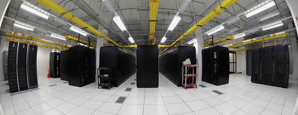
Cloud (Data Center) Architectures with physical setup, Green Computing issues and software models are discussed followed by the Cloud Industry stakeholders with a 2014 Gartner analysis of Cloud computing providers. This is followed by applications on the cloud including data intensive problems, comparison with high performance computing, science clouds and the Internet of Things. Remarks on Security, Fault Tolerance and Synchronicity issues in cloud follow. We describe the way users and data interact with a cloud system. The Big Data Processing from an application perspective with commercial examples including eBay concludes section after a discussion of data system architectures.
Geoffrey describes the central role of Parallel computing in Clouds and Big Data which is decomposed into lots of ''Little data'' running in individual cores. Many examples are given and it is stressed that issues in parallel computing are seen in day to day life for communication, synchronization, load balancing and decomposition.
Geoffrey describes why parallel computing is essential with Big Data and distinguishes parallelism over users to that over the data in problem. The general ideas behind data decomposition are given followed by a few often whimsical examples dreamed up 30 years ago in the early heady days of parallel computing. These include scientific simulations, defense outside missile attack and computer chess. The basic problem of parallel computing -- efficient coordination of separate tasks processing different data parts -- is described with MPI and MapReduce as two approaches. The challenges of data decomposition in irregular problems is noted.
Geoffrey describes why parallel computing is essential with Big Data and distinguishes parallelism over users to that over the data in problem. The general ideas behind data decomposition are given followed by a few often whimsical examples dreamed up 30 years ago in the early heady days of parallel computing. These include scientific simulations, defense outside missile attack and computer chess. The basic problem of parallel computing -- efficient coordination of separate tasks processing different data parts -- is described with MPI and MapReduce as two approaches. The challenges of data decomposition in irregular problems is noted.
Geoffrey describes why parallel computing is essential with Big Data and distinguishes parallelism over users to that over the data in problem. The general ideas behind data decomposition are given followed by a few often whimsical examples dreamed up 30 years ago in the early heady days of parallel computing. These include scientific simulations, defense outside missile attack and computer chess. The basic problem of parallel computing -- efficient coordination of separate tasks processing different data parts -- is described with MPI and MapReduce as two approaches. The challenges of data decomposition in irregular problems is noted.
This lesson from the past notes that one can view society as an approach to parallel linkage of people. The largest example given is that of the construction of a long wall such as that (Hadrian's wall) between England and Scotland. Different approaches to parallelism are given with formulae for the speed up and efficiency. The concepts of grain size (size of problem tackled by an individual processor) and coordination overhead are exemplified. This example also illustrates Amdahl's law and the relation between data and processor topology. The lesson concludes with other examples from nature including collections of neurons (the brain) and ants.
This lesson from the past notes that one can view society as an approach to parallel linkage of people. The largest example given is that of the construction of a long wall such as that (Hadrian's wall) between England and Scotland. Different approaches to parallelism are given with formulae for the speed up and efficiency. The concepts of grain size (size of problem tackled by an individual processor) and coordination overhead are exemplified. This example also illustrates Amdahl's law and the relation between data and processor topology. The lesson concludes with other examples from nature including collections of neurons (the brain) and ants.
This lesson returns to Hadrian's wall and uses it to illustrate advanced issues in parallel computing. First Geoffrey describes the basic SPMD -- Single Program Multiple Data -- model. Then irregular but homogeneous and heterogeneous problems are discussed. Static and dynamic load balancing is needed. Inner parallelism (as in vector instruction or the multiple fingers of masons) and outer parallelism (typical data parallelism) are demonstrated. Parallel I/O for Hadrian's wall is followed by a slide summarizing this quaint comparison between Big data parallelism and the construction of a large wall.
Geoffrey discusses Cyberinfrastructure for e-moreorlessanything or moreorlessanything-Informatics and the basics of cloud computing. This includes virtualization and the important 'as a Service' components and we go through several different definitions of cloud computing.
Gartner's Technology Landscape includes hype cycle and priority matrix and covers clouds and Big Data. The unit concludes with two simple examples of the value of clouds for enterprise applications. Gartner also has specific predictions for cloud computing growth areas.
This introduction describes Cyberinfrastructure or e-infrastructure and its role in solving the electronic implementation of any problem where e-moreorlessanything is another term for moreorlessanything-Informatics and generalizes early discussion of e-Science and e-Business.
Cloud Computing is introduced with an operational definition involving virtualization and efficient large data centers that can rent computers in an elastic fashion. The role of services is essential -- it underlies capabilities being offered in the cloud. The four basic aaS's -- Software (SaaS), Platform (Paas), Infrastructure (IaaS) and Network (NaaS) -- are introduced with Research aaS and other capabilities (for example Sensors aaS are discussed later) being built on top of these.
This lesson contains 5 slides with diverse comments on ''what is cloud computing'' from the web.
This lesson contains 5 slides with diverse comments on ''what is cloud computing'' from the web.
This lesson contains 5 slides with diverse comments on ''what is cloud computing'' from the web.
This lesson gives Gartner's projections around futures of cloud and Big data. We start with a review of hype charts and then go into detailed Gartner analyses of the Cloud and Big data areas. Big data itself is at the top of the hype and by definition predictions of doom are emerging. Before too much excitement sets in, note that spinach is above clouds and Big data in Google trends.
This short lesson gives two examples of rather straightforward commercial applications of cloud computing. One is server consolidation for multiple Microsoft database applications and the second is the benefits of scale comparing gmail to multiple smaller installations. It ends with some fiscal comments
Some comments on fiscal value of cloud computing
Geoffrey covers different views as to nature of architecture and application for Cloud Computing. Then we discuss cloud software for the cloud starting at virtual machine management (IaaS) and the broad Platform (middleware) capabilities with examples from Amazon and academic studies. We summarize the 21 layers and almost 300 software packages in the HPC-ABDS Software Stack explaining how they are used.
This lesson gives some general remark of cloud systems from an architecture and application perspective.
Geoffrey discusses cloud software for the cloud starting at virtual machine management (IaaS) and the broad Platform (middleware) capabilities with examples from Amazon and academic studies.
Geoffrey discusses cloud software for the cloud starting at virtual machine management (IaaS) and the broad Platform (middleware) capabilities with examples from Amazon and academic studies.
Using the HPC-ABDS Software Stack.
Geoffrey opens up with a discussion of Cloud (Data Center) Architectures with physical setup, Green Computing issues and software models. We summarize a 2014 Gartner analysis of Cloud computing providers. This is followed by applications on the cloud including data intensive problems, comparison with high performance computing, science clouds and the Internet of Things. Remarks on Security, Fault Tolerance and Synchronicity issues in cloud follow.
Some remarks on what it takes to build (in software) a cloud ecosystem, and why clouds are the data center of the future are followed by pictures and discussions of several data centers from Microsoft (mainly) and Google. The role of containers is stressed as part of modular data centers that trade scalability for fault tolerance. Sizes of cloud centers and supercomputers are discussed as is ''green'' computing.
Some remarks on what it takes to build (in software) a cloud ecosystem, and why clouds are the data center of the future are followed by pictures and discussions of several data centers from Microsoft (mainly) and Google. The role of containers is stressed as part of modular data centers that trade scalability for fault tolerance. Sizes of cloud centers and supercomputers are discussed as is ''green'' computing.
Gartner 2014 Analysis of leading cloud providers.
Use of Dropbox, iCloud, Box etc.
This short lesson discusses the need for security and issues in its implementation.
Clouds trade scalability for greater possibility of faults but here clouds offer good support for recovery from faults. We discuss both storage and program fault tolerance noting that parallel computing is especially sensitive to faults as a fault in one task will impact all other tasks in the parallel job.
Science Applications and Internet of Things.
This short lesson discusses the need for security and issues in its implementation.
Clouds trade scalability for greater possibility of faults but here clouds offer good support for recovery from faults. We discuss both storage and program fault tolerance noting that parallel computing is especially sensitive to faults as a fault in one task will impact all other tasks in the parallel job.
We describe the way users and data interact with a cloud system. The unit concludes with the treatment of data in the cloud from an architecture perspective and Big Data Processing from an application perspective with commercial examples including eBay.
The next 3 lessons describe the way users and data interact with the system.
This lessons describe the way users and data interact with the system for some science examples.
This lesson describe the way users and data interact with the system for the final set of examples.
Databases, File systems, Object Stores and NOSQL are discussed and compared. The way to build a modern data repository in the cloud is introduced.
This lesson collects remarks on Big data processing from several sources: Berkeley, Teradata, IBM, Oracle and eBay with architectures and application opportunities.

This section starts with an overview of data mining and puts our study of classification, clustering and exploration methods in context. We examine the problem to be solved in web and text search and note the relevance of history with libraries, catalogs and concordances. An overview of web search is given describing the continued evolution of search engines and the relation to the field of Information Retrieval. The importance of recall, precision and diversity is discussed. The important Bag of Words model is introduced and both Boolean queries and the more general fuzzy indices. The important vector space model and revisiting the Cosine Similarity as a distance in this bag follows. The basic TF-IDF approach is dis cussed. Relevance is discussed with a probabilistic model while the distinction between Bayesian and frequency views of probability distribution completes this unit. Geoffrey starts with an overview of the different steps (data analytics) in web search and then goes key steps in detail starting with document preparation. An inverted index is described and then how it is prepared for web search. The Boolean and Vector Space approach to query processing follow. This is followed by Link Structure Analysis including Hubs, Authorities and PageRank. The application of PageRank ideas as reputation outside web search is covered. The web graph structure, crawling it and issues in web advertising and search follow. The use of clustering and topic models completes section.
The unit starts with the web with its size, shape (coming from the mutual linkage of pages by URL's) and universal power laws for number of pages with particular number of URL's linking out or in to page. Information retrieval is introduced and compared to web search. A comparison is given between semantic searches as in databases and the full text search that is base of Web search. The origin of web search in libraries, catalogs and concordances is summarized. DIKW -- Data Information Knowledge Wisdom -- model for web search is discussed. Then features of documents, collections and the important Bag of Words representation. Queries are presented in context of an Information Retrieval architecture. The method of judging quality of results including recall, precision and diversity is described. A time line for evolution of search engines is given.
Boolean and Vector Space models for query including the cosine similarity are introduced. Web Crawlers are discussed and then the steps needed to analyze data from Web and produce a set of terms. Building and accessing an inverted index is followed by the importance of term specificity and how it is captured in TF-IDF. We note how frequencies are converted into belief and relevance
This lesson starts with the web with its size, shape (coming from the mutual linkage of pages by URL's) and universal power laws for number of pages with particular number of URL's linking out or in to page.
Information retrieval is introduced A comparison is given between semantic searches as in databases and the full text search that is base of Web search. The ACM classification illustrates potential complexity of ontologies. Some differences between web search and information retrieval are given.
The origin of web search in libraries, catalogs and concordances is summarized.
This lesson describes the DIKW -- Data Information Knowledge Wisdom -- model for web search. Then it discusses documents, collections and the important Bag of Words representation.
This describes queries in context of an Information Retrieval architecture. The method of judging quality of results including recall, precision and diversity is described.
This short lesson describes a time line for evolution of search engines. The first web search approaches were directly built on Information retrieval but in 1998 the field was changed when Google was founded and showed the importance of URL structure as exemplified by PageRank.
This lesson describes the Boolean and Vector Space models for query including the cosine similarity
This describes a Web Crawler and then the steps needed to analyze data from Web and produce a set of terms
This lesson describes both building and accessing an inverted index. It describes how phrases are treated and gives details of query structure from some early logs
It describes the importance of term specificity and how it is captured in TF-IDF. It notes how frequencies are converted into belief and relevance
Geoffrey starts with an overview of the different steps (data analytics) in web search. This is followed by Link Structure Analysis including Hubs, Authorities and PageRank. The application of PageRank ideas as reputation outside web search is covered. Issues in web advertising and search follow. his leads to emerging field of computational advertising. The use of clustering and topic models completes unit with Google News as an example.
This short lesson describes the different steps needed in web search including: Get the digital data (from web or from scanning); Crawl web; Preprocess data to get searchable things (words, positions); Form Inverted Index mapping words to documents; Rank relevance of documents with potentially sophisticated techniques; and integrate technology to support advertising and ways to allow or stop pages artificially enhancing relevance.
The value of links and the concepts of Hubs and Authorities are discussed. This leads to definition of PageRank with examples. Extensions of PageRank viewed as a reputation are discussed with journal rankings and university department rankings as examples. There are many extension of these ideas which are not discussed here although topic models are covered briefly in a later lesson.
The value of links and the concepts of Hubs and Authorities are discussed. This leads to definition of PageRank with examples. Extensions of PageRank viewed as a reputation are discussed with journal rankings and university department rankings as examples. There are many extension of these ideas which are not discussed here although topic models are covered briefly in a later lesson.
Internet and mobile advertising is growing fast and can be personalized more than for traditional media. There are several advertising types Sponsored search, Contextual ads, Display ads and different models: Cost per viewing, cost per clicking and cost per action. This leads to emerging field of computational advertising.
We discuss briefly approaches to defining groups of documents. We illustrate this for Google News and give an example that this can give different answers from word-based analyses. We mention some work at Indiana University on a Latent Semantic Indexing model.

Geoffrey uses the K-means Python code in SciPy package to show real code for clustering. After a simple example we generate 4 clusters of distinct centers and various choice for sizes using Matplotlib tor visualization. We show results can sometimes be incorrect and sometimes make different choices among comparable solutions. We discuss the ''hill'' between different solutions and rationale for running K-means many times and choosing best answer. Then we introduce MapReduce with the basic architecture and a homely example. The discussion of advanced topics includes an extension to Iterative MapReduce from Indiana University called Twister and a generalized Map Collective model. Some measurements of parallel performance are given. The SciPy K-means code is modified to support a MapReduce execution style. This illustrates the key ideas of mappers and reducers. With appropriate runtime this code would run in parallel but here the ''parallel'' maps run sequentially. This simple 2 map version can be generalized to scalable parallelism. Python is used to Calculate PageRank from Web Linkage Matrix showing several different formulations of the basic matrix equations to finding leading eigenvector. The unit is concluded by a calculation of PageRank for general web pages by extracting the secret from Google.
Geoffrey uses the K-means Python code in SciPy package to show real code for clustering. After a simple example we generate 4 clusters of distinct centers and various choice for sizes using Matplotlib tor visualization. We show results can sometimes be incorrect and sometimes make different choices among comparable solutions. We discuss the ''hill'' between different solutions and rationale for running K-means many times and choosing best answer.
Geoffrey uses the K-means Python code in SciPy package to show real code for clustering and applies it a set of 85 two dimensional vectors -- officially sets of weights and heights to be clustered to find T-shirt sizes. We run through Python code with Matplotlib displays to divide into 2-5 clusters. Then we discuss Python to generate 4 clusters of varying sizes and centered at corners of a square in two dimensions. We formally give the K means algorithm better than before and make definition consistent with code in SciPy
We present clustering results on the artificial set of 1000 2D points described in previous lesson for 3 choices of cluster sizes ''small'' ''large'' and ''very large''. We emphasize the SciPy always does 20 independent K means and takes the best result -- an approach to avoiding local minima. We allow this number of independent runs to be changed and in particular set to 1 to generate more interesting erratic results. We define changes in our new K means code that also has two measures of quality allowed. The slides give many results of clustering into 2 4 6 and 8 clusters (there were only 4 real clusters). We show that the ''very small'' case has two very different solutions when clustered into two clusters and use this to discuss functions with multiple minima and a hill between them. The lesson has both discussion of already produced results in slides and interactive use of Python for new runs.
We present clustering results on the artificial set of 1000 2D points described in previous lesson for 3 choices of cluster sizes ''small'' ''large'' and ''very large''. We emphasize the SciPy always does 20 independent K means and takes the best result -- an approach to avoiding local minima. We allow this number of independent runs to be changed and in particular set to 1 to generate more interesting erratic results. We define changes in our new K means code that also has two measures of quality allowed. The slides give many results of clustering into 2 4 6 and 8 clusters (there were only 4 real clusters). We show that the ''very small'' case has two very different solutions when clustered into two clusters and use this to discuss functions with multiple minima and a hill between them. The lesson has both discussion of already produced results in slides and interactive use of Python for new runs.
We present clustering results on the artificial set of 1000 2D points described in previous lesson for 3 choices of cluster sizes ''small'' ''large'' and ''very large''. We emphasize the SciPy always does 20 independent K means and takes the best result -- an approach to avoiding local minima. We allow this number of independent runs to be changed and in particular set to 1 to generate more interesting erratic results. We define changes in our new K means code that also has two measures of quality allowed. The slides give many results of clustering into 2 4 6 and 8 clusters (there were only 4 real clusters). We show that the ''very small'' case has two very different solutions when clustered into two clusters and use this to discuss functions with multiple minima and a hill between them. The lesson has both discussion of already produced results in slides and interactive use of Python for new runs.
Geoffrey's introduction to MapReduce describes the basic architecture and a homely example. The discussion of advanced topics includes extension to Iterative MapReduce from Indiana University called Twister and a generalized Map Collective model. Some measurements of parallel performance are given
This introduction uses an analogy to making fruit punch by slicing and blending fruit to illustrate MapReduce. The formal structure of MapReduce and Iterative MapReduce is presented with parallel data flowing from disks through multiple Map and Reduce phases to be inspected by the user
This defines 4 types of MapReduce and the Map Collective model of Qiu. The Iterative MapReduce model from Indiana University called Twister is described and a few performance measurements on Microsoft Azure are presented.
This defines 4 types of MapReduce and the Map Collective model of Qiu. The Iterative MapReduce model from Indiana University called Twister is described and a few performance measurements on Microsoft Azure are presented.
Geoffrey modifies the SciPy K-means code to support a MapReduce execution style and runs it in this short unit. This illustrates the key ideas of mappers and reducers. With appropriate runtime this code would run in parallel but here the ''parallel'' maps run sequentially. Geoffrey stresses that this simple 2 map version can be generalized to scalable parallelism.
Geoffrey modifies the SciPy K-means code to support a MapReduce execution style and runs it in this short unit. This illustrates the key ideas of mappers and reducers. With appropriate runtime this code would run in parallel but here the ''parallel'' maps run sequentially. Geoffrey stresses that this simple 2 map version can be generalized to scalable parallelism.
Geoffrey modifies the SciPy K-means code to support a MapReduce execution style and runs it in this short unit. This illustrates the key ideas of mappers and reducers. With appropriate runtime this code would run in parallel but here the ''parallel'' maps run sequentially. Geoffrey stresses that this simple 2 map version can be generalized to scalable parallelism.
Geoffrey uses Python to Calculate PageRank from Web Linkage Matrix showing several different formulations of the basic matrix equations to finding leading eigenvector. The unit is concluded by a calculation of PageRank for general web pages by extracting the secret from Google.
Geoffrey takes two simple matrices for 6 and 8 web sites respectively to illustrate the calculation of PageRank.
Geoffrey takes two simple matrices for 6 and 8 web sites respectively to illustrate the calculation of PageRank.
This tiny lesson presents a Python code that finds the Page Rank that Google calculates for any page on the web

Sports sees significant growth in analytics with pervasive statistics shifting to more sophisticated measures. We start with baseball as game is built around segments dominated by individuals where detailed (video/image) achievement measures including PITCHf/x and FIELDf/x are moving field into big data arena. There are interesting relationships between the economics of sports and big data analytics. We look at Wearables and consumer sports/recreation. The importance of spatial visualization is discussed. We look at other Sports: Soccer, Olympics, NFL Football, Basketball, Tennis and Horse Racing.
This unit discusses baseball starting with the movie Moneyball and the 2002-2003 Oakland Athletics. Unlike sports like basketball and soccer, most baseball action is built around individuals often interacting in pairs. This is much easier to quantify than many player phenomena in other sports. We discuss Performance-Dollar relationship including new stadiums and media/advertising. We look at classic baseball averages and sophisticated measures like Wins Above Replacement.
Introduction to all Sports Informatics, Moneyball The 2002-2003 Oakland Athletics, Diamond Dollars economic model of baseball, Performance - Dollar relationship, Value of a Win.
Different Types of Baseball Data, Sabermetrics, Overview of all data, Details of some statistics based on basic data, OPS, wOBA, ERA, ERC, FIP, UZR.
Wins above Replacement WAR, Discussion of Calculation, Examples, Comparisons of different methods, Coefficient of Determination, Another, Sabermetrics Example, Summary of Sabermetrics.
This unit discusses 'advanced sabermetrics' covering advances possible from using video from PITCHf/X, FIELDf/X, HITf/X, COMMANDf/X and MLBAM.
A Big Data Pitcher Clustering method introduced by Vince Gennaro, Data from Blog and video at 2013 SABR conference.
Results of optimizing match ups, Data from video at 2013 SABR conference.
Examples of use of PITCHf/X.
FIELDf/X, MLBAM, HITf/X, COMMANDf/X.
We look at Wearables and consumer sports/recreation. The importance of spatial visualization is discussed. We look at other Sports: Soccer, Olympics, NFL Football, Basketball, Tennis and Horse Racing.
Consumer Sports, Stake Holders, and Multiple Factors.
Soccer, Tracking Players and Balls, Olympics.
NFL, NBA, and Spatial Visualization.
Tennis, Horse Racing, and Continued Emphasis on Spatial Visualization.

This section starts by discussing general aspects of Big Data and Health including data sizes, different areas including genomics, EBI, radiology and the Quantified Self movement. We review current state of health care and trends associated with it including increased use of Telemedicine. We summarize an industry survey by GE and Accenture and an impressive exemplar Cloud-based medicine system from Potsdam. We give some details of big data in medicine. Some remarks on Cloud computing and Health focus on security and privacy issues. We survey an April 2013 McKinsey report on the Big Data revolution in US health care; a Microsoft report in this area and a European Union report on how Big Data will allow patient centered care in the future. Examples are given of the Internet of Things, which will have great impact on health including wearables. A study looks at 4 scenarios for healthcare in 2032. Two are positive, one middle of the road and one negative. The final topic is Genomics, Proteomics and Information Visualization.
This section starts by discussing general aspects of Big Data and Health including data sizes, different areas including genomics, EBI, radiology and the Quantified Self movement. We review current state of health care and trends associated with it including increased use of Telemedicine. We summarize an industry survey by GE and Accenture and an impressive exemplar Cloud-based medicine system from Potsdam. We give some details of big data in medicine. Some remarks on Cloud computing and Health focus on security and privacy issues. We survey an April 2013 McKinsey report on the Big Data revolution in US health care; a Microsoft report in this area and a European Union report on how Big Data will allow patient centered care in the future. Examples are given of the Internet of Things, which will have great impact on health including wearables. A study looks at 4 scenarios for healthcare in 2032. Two are positive, one middle of the road and one negative. The final topic is Genomics, Proteomics and Information Visualization.
This lesson starts with general aspects of Big Data and Health including listing subareas where Big data important. Data sizes are given in radiology, genomics, personalized medicine, and the Quantified Self movement, with sizes and access to European Bioinformatics Institute.
This covers trends of costs and type of healthcare with low cost genomes and an aging population. Social media and government Brain initiative.
This describes increasing use of telemedicine and how we tried and failed to do this in 1994.
Summary of an industry survey by GE and Accenture.
An impressive exemplar Cloud-based medicine system from Potsdam.
This lesson starts with a look at a start up using clouds in Health/Medical informatics. Then we review an online presentation on Healthcare and clouds. Conforming with HIPAA act is important. Advantages of clouds include low cost and ease of anywhere access and convenience of sharing information. Security and privacy are main problem area.
This lesson covers 9 aspects of the McKinsey report. These are the convergence of multiple positive changes has created a tipping point for innovation; Primary data pools are at the heart of the big data revolution in healthcare; Big data is changing the paradigm: these are the value pathways; Applying early successes at scale could reduce US healthcare costs by $300 billion to $450 billion; Most new big-data applications target consumers and providers across pathways; Innovations are weighted towards influencing individual decision-making levers; Big data innovations use a range of public, acquired, and proprietary data types; Organizations implementing a big data transformation should provide the leadership required for the associated cultural transformation; Companies must develop a range of big data capabilities
This lesson identifies data sources as Clinical Data, Pharma & Life Science Data, Patient & Consumer Data, Claims & Cost Data and Correlational Data. Three approaches are Live data feed, Advanced analytics and Social analytics.
This lesson summarizes an EU Report on Redesigning health in Europe for 2020. The power of data is seen as a lever for change in My Data, My decisions; Liberate the data; Connect up everything; Revolutionize health; and Include Everyone removing the current correlation between health and wealth.
The Internet of Things will have great impact on health including telemedicine and wearables. Examples are given.
A study looks at 4 scenarios for healthcare in 2032. Two are positive, one middle of the road and one negative.
A study of an Azure application with an Excel frontend and a cloud BLAST backend starts this lesson. This is followed by a big data analysis of personal genomics and an analysis of a typical DNA sequencing analytics pipeline. The Protein Sequence Universe is defined and used to motivate Multi dimensional Scaling MDS. Sammon's method is defined and its use illustrated by a metagenomics example. Subtleties in use of MDS include a monotonic mapping of the dissimilarity function. The application to the COG Proteomics dataset is discussed. We note that the MDS approach is related to the well known chisq method and some aspects of nonlinear minimization of chisq (Least Squares) are discussed.
This lesson continues the discussion of the COG Protein Universe introduced in the last lesson. It is shown how Proteomics clusters are clearly seen in the Universe browser. This motivates a side remark on different clustering methods applied to metagenomics. Then we discuss the Generative Topographic Map GTM method that can be used in dimension reduction when original data is in a metric space and is in this case faster than MDS as GTM computational complexity scales like N not N squared as seen in MDS. Examples are given of GTM including an application to topic models in Information Retrieval. Indiana University has developed a deterministic annealing improvement of GTM. 3 separate clusterings are projected for visualization and show very different structure emphasizing the importance of visualizing results of data analytics. The final slide shows an application of MDS to generate and visualize phylogenetic trees.
This lesson continues the discussion of the COG Protein Universe introduced in the last lesson. It is shown how Proteomics clusters are clearly seen in the Universe browser. This motivates a side remark on different clustering methods applied to metagenomics. Then we discuss the Generative Topographic Map GTM method that can be used in dimension reduction when original data is in a metric space and is in this case faster than MDS as GTM computational complexity scales like N not N squared as seen in MDS. Examples are given of GTM including an application to topic models in Information Retrieval. Indiana University has developed a deterministic annealing improvement of GTM. 3 separate clusterings are projected for visualization and show very different structure emphasizing the importance of visualizing results of data analytics. The final slide shows an application of MDS to generate and visualize phylogenetic trees.

Geoffrey starts with the Internet of Things IoT giving examples like monitors of machine operation, QR codes, surveillance cameras, scientific sensors, drones and self driving cars and more generally transportation systems. We give examples of robots and drones. We introduce the Industrial Internet of Things IIoT and summarize surveys and expectations Industry wide. We give examples from General Electric. Sensor clouds control the many small distributed devices of IoT and IIoT. More detail is given for radar data gathered by sensors; ubiquitous or smart cities and homes including U-Korea; and finally the smart electric grid.
Geoffrey starts with the Internet of Things IoT giving examples like monitors of machine operation, QR codes, surveillance cameras, scientific sensors, drones and self driving cars and more generally transportation systems. We give examples of robots and drones. We introduce the Industrial Internet of Things IIoT and summarize surveys and expectations Industry wide. We give examples from General Electric. Sensor clouds control the many small distributed devices of IoT and IIoT. More detail is given for radar data gathered by sensors; ubiquitous or smart cities and homes including U-Korea; and finally the smart electric grid.
There are predicted to be 24-50 Billion devices on the Internet by 2020; these are typically some sort of sensor defined as any source or sink of time series data. Sensors include smartphones, webcams, monitors of machine operation, barcodes, surveillance cameras, scientific sensors (especially in earth and environmental science), drones and self driving cars and more generally transportation systems. The lesson gives many examples of distributed sensors, which form a Grid that is controlled by a cloud.
Examples of Robots and Drones.
We summarize surveys and expectations Industry wide.
Examples from General Electric.
Geoffrey describes the architecture of a Sensor Cloud control environment and gives example of interface to an older version of it. The performance of system is measured in terms of processing latency as a function of number of involved sensors with each delivering data at 1.8 Mbps rate.
This lesson gives examples of some sensors in the Earth/Environment/Polar Science field. It starts with material from the CReSIS polar remote sensing project and then looks at the NSF Ocean Observing Initiative and NASA's MODIS or Moderate Resolution Imaging Spectroradiometer instrument on a satellite.
For Ubiquitous/Smart cities we give two examples: Iniquitous Korea and smart electrical grids
Korea has an interesting positioning where it is first worldwide in broadband access per capita, e-government, scientific literacy and total working hours. However it is far down in measures like quality of life and GDP. U-Korea aims to improve the latter by Pervasive computing, everywhere, anytime i.e. by spreading sensors everywhere. The example of a 'High-Tech Utopia' New Songdo is given.
The electrical Smart Grid aims to enhance USA's aging electrical infrastructure by pervasive deployment of sensors and the integration of their measurement in a cloud or equivalent server infrastructure. A variety of new instruments include smart meters, power monitors, and measures of solar irradiance, wind speed, and temperature. One goal is autonomous local power units where good use is made of waste heat.

The changing global climate is suspected to have long-term effects on much of the world's inhabitants. Among the various effects, the rising sea level will directly affect many people living in low-lying coastal regions. While the ocean-s thermal expansion has been the dominant contributor to rises in sea level, the potential contribution of discharges from the polar ice sheets in Greenland and Antarctica may provide a more significant threat due to the unpredictable response to the changing climate. The Radar-Informatics unit provides a glimpse in the processes fueling global climate change and explains what methods are used for ice data acquisitions and analysis.
This unit motivates radar-informatics by building on previous discussions on why X-applications are growing in data size and why analytics are necessary for acquiring knowledge from large data. The unit details three mosaics of a changing Greenland ice sheet and provides a concise overview to subsequent lessons by detailing explaining how other remote sensing technologies, such as the radar, can be used to sound the polar ice sheets and what we are doing with radar images to extract knowledge to be incorporated into numerical models.
This explains the basics of remote sensing, the characteristics of remote sensors and remote sensing applications. Emphasis is on image acquisition and data collection in the electromagnetic spectrum.
This unit provides a brief understanding on why melt water at the base of the ice sheet can be detrimental and why it’s important for sensors to sound the bedrock.
This unit provides an understanding and the processes for the greenhouse effect, how warming effects the Polar Regions, and the implications of a rise in sea level.
This unit provides an elementary introduction to radar and its importance to remote sensing, especially to acquiring information about Greenland and Antarctica.
This unit focuses on the use of sophisticated computer vision algorithms, such as active contours and a hidden markov model to support data analysis for extracting layers, so ice sheet models can accurately forecast future changes in climate.